

Google’s Vertex AI and AutoML - create a model and obtain predictions
Useful links:
This article refers to tables and data seen in this article
From the data in the training table we created and what we’ll give Vertex AI (columns we want to take into account, how…) we will create a model that we can use to predict future sales.
This process takes some time, depending on the number of rows of the dataset. Here, with approximately 20 million rows, obtaining the model takes about an hour.
Train a new model
Training method
Go to the Vertex AI tab of the Google Console and choose the training menu. Create a new model. This window will appear:
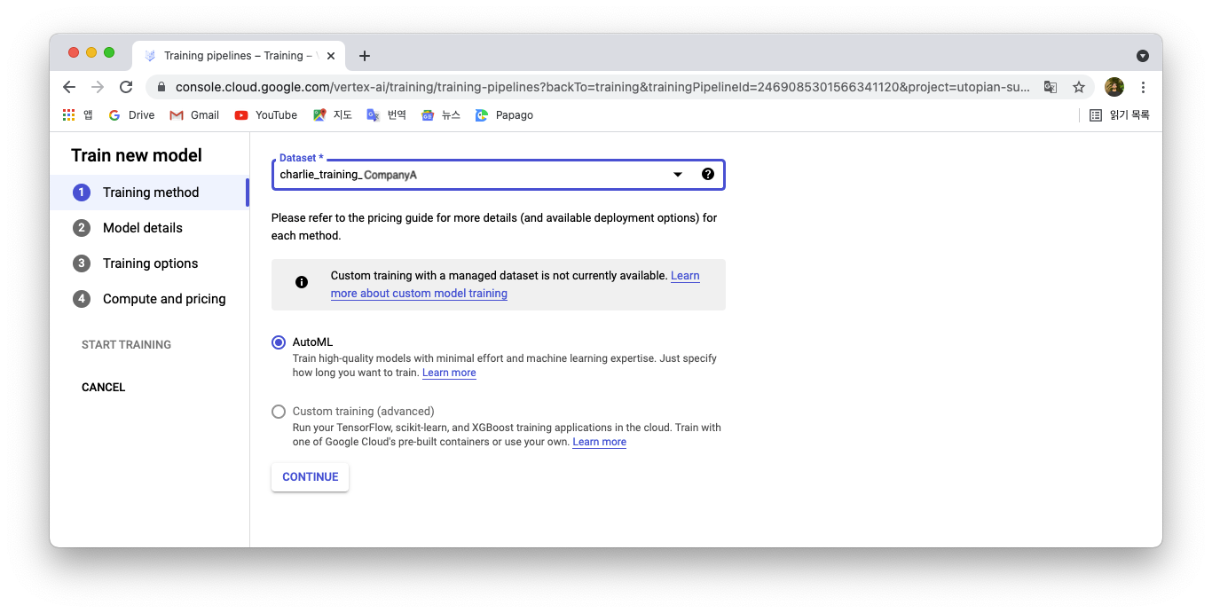
Choose the right dataset and select AutoML. Google’s AutoML is the best option here as the custom training requires a lot of code writing and is more time consuming. After clicking on continue, we’ll have to provide the necessary details about our dataset so Vertex AI’s AutoML can build an efficient model.
Model details
Here we specify the role of our columns, you can select them from a list :
- Model name : It can be anything
- Target column : The column we want the data predicted for, SALES_2C
- Time series identifier column (TSID) : The row item you want to be predicted. You could choose to predict the sales of a certain product per store, or just the sales of an item. Here, we’ll go with predictions of an item, regardless of country, store etc. The data should be prepared accordingly : see the Vertex AI documentation
- Timestamp column : We’re predicting a time series, so we need a time dimension.
- Data granularity : In our data set, we have weekly data. The “step” of our timestamps is 1 week. In other datasets, it could be daily, hourly…
- Forecast horizon : In the same unit as the data granularity, it lets you choose how far in the future the data should be predicted. 10 weeks is a good horizon.
- Context window : Again, in the same unit as the data granularity, how far back should Vertex AI look to build the model. Usually, the context window and forecast horizon are of the same length. So here we choose 10 as well.
Other settings, such as export test dataset to BigQuery, data validation options, daata split, can be left on the default choice.
Training options
Feature type
We have to attribute a feature type to each column: they can be either attribute or covariate. If the column corresponds to an element that doesnt really evolve or change over time, it is an attribute (e.g. product id) if it is deemed to change and evlove, it is a covariate (e.g. sales, date…)
Available at forecast
Then the Available at forecast refers to the data we have available already in the future: we already the know the seasonality effect of Christmas, so it is available at forecast. Same goes for the product id. The data we’re trying to predict (sales) obviously isn’t available.
Weight columns
Weight columns allows to give a bigger importance to a certain column. If in the data we’re trying to predict seasonality has a specifically strong influence, then we can give it extra weight.
Optimization objective
This is how we want our error margin to be evaluated, and corrected. MAE (Mean Average Error) is a good place to start. Based on a mean principle, the more extreme values will be considered “exceptional” and be considered less relevant to the prediction.
Compute and pricing
Node hours
According to the number of rows, there are recommended node hours amount. Here, because it’s for practice, we’ll go the lowest with 1 node hour.
This is where we can also see the pricing for this training model. As of august 2021, for tabular prediction, 1 node hour is billed a little under USD20.
We can now train our model, and get one step closer to obtain sales predictions for Company A!
Obtain a prediction
After the training is done and the model is created, we can go to the next step and obtain our predicted data.
In the training menu, the name of the model we chose earlier should be appearing, preceded by a green checkmark ✅. Click on your model name: a new window appears with 3 tabs: Evaluate, Batch predictions and Model properties.
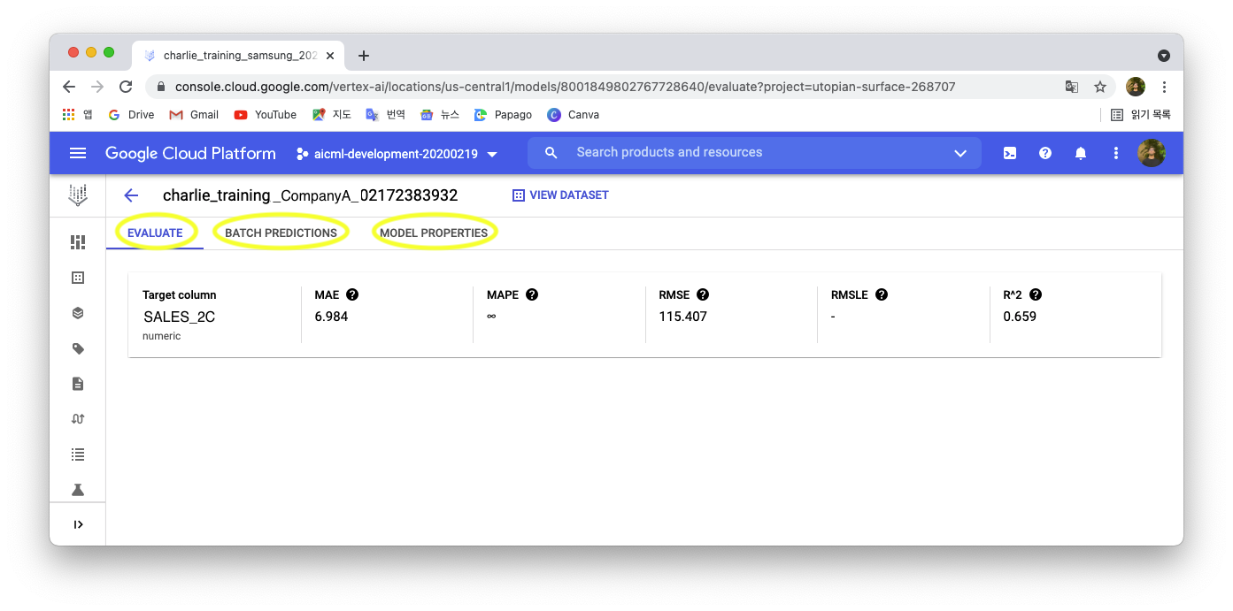
To obtain the predictions, we must create a new batch prediction: we’ll click on the BATCH PREDICTIONS tab and fill in the fields as follows in the new menu that opened.
New batch prediction
We’ll be using the table made in the previous article as our “input table” 1.
- Batch prediction name : any name that works for the final prediction table
- Model name : should be already filled in with the model we’ve just made
- Select source : We’ll feed the table input table mention above , so we’ll put:
- Google Cloud Project ID:
utopian-surface-268707 - BigQuery dataset ID:
Charlie_uscentral1 - BigQuery table or view ID:
CompanyA_predict_table_unionized
- Google Cloud Project ID:
- Output format : BigQuery
- BigQuery path : to have our predictions in the same dataset as the other tables:
utopian-surface-268707.Charlie_uscentral1. It is also possible to create a new dataset by simply entering the Project ID, it will be automatically created.
After clicking on Create batch prediction, the sales prediction will start, which takes around 20mns for our table. Once done, on the model’s batch predictions menu, our freshly made table will appear with a green check ✅ next to it. We can open it in BigQuery directly by clicking on it and then on the link next to Export location in the table.
Depending on the input table, there might be errors. In our errors correspond to the “past data” that wasn’t nulled. We can ignore this and focus on the predictions made in the other table of the data set. In the scheme of that table, we can see that a new column was created: predicted_SALES_2C. This column contains the newly predicted sales data.
Looking at the table in the preview view, data is too complicated to be understood. In order to take advantage of the predictions we’ve just made, and have it understood by everyone, we can summarize it in a graph. We’ll see how we can do that using Google Data Studio in the next article.
1 It is very important that SALES_2C, SALES_2B, STOCK columns have null values.
Thank you Kylie for your help in making this!