

Starting up with GCP and SQL
Useful links:
BigQuery and Datasets
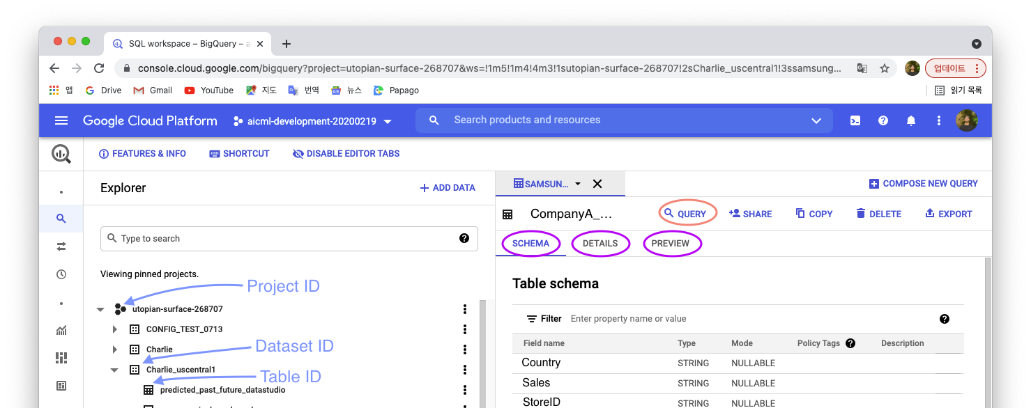
From the tab on the left click on BigQuery, a list of project appears on left, choose one and create a dataset if necessary, add data to it, in the form of a table - CSV file for exemple.
GCP accepts following files to import a table:
- CSV
- JSON
- AVRO
- Parquet
- ORC
After the table is imported it is ready to be used, queried in BigQuery.
View, format and wrangle tables in BigQuery
There are 3 tabs after you open a table in GCP’s BigQuery editor:
- Schema: See the columns/features of your table in a list form, with information about their type
- Details: See informations about the Table: ID, size, number of rows…
- Preview: See your CSV file converted into a table format
To start a new Query, click on the Query button on the top right of the screen.
The window divides in two and an SQL environment opens. It should look like something like this:
SELECT FROM `YOUR TABLE ID` LIMIT 1000
-
SELECT: allows you to select specific columns to visualize after processing your Query.*to visualize all columns. -
FROM: is what tells the environment where to look for selected columns -
LIMIT: allows to set a limit of number of rows after which the Query won’t process.
With for example the Company A data, we only want to see countries, product, sales 2 business, sales 2 customer and seasonality:
Each column name should be separated by a comma:
SELECT
Country,
Productid,
Sales_2C,
Sales_2B,
Seasonality
FROM `utopian-surface-268707.Charlie_uscentral1.CompanyA_origin_29w`
-- Limit not necessary, we want all data to be sorted through.
We can now run the query, press RUN or keybord shortcut ⌘ + ↵.
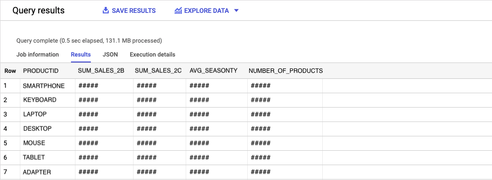
The table appears in bottom left corner and we should be able to see only the columns we’ve selected. Now, maybe it would be more interesting to sort the table and group the PRODUCTIDs by products.
SELECT
  PRODUCTID,
  cast(sum (Sales_2C) as STRING FORMAT '999,999,999.99') as SUM_SALES_2C,
  cast(sum (Sales_2B) as STRING FORMAT '999,999,999.99') as SUM_SALES_2B,
  avg (Seasonality) as AVG_SEASONTY,
  count(*) as NUMBER_OF_PRODUCTS,
  FROM
  `utopian-surface-268707.Charlie_uscentral1.CompanyA_origin_29w`
group by PRODUCTID
order by PRODUCTID
Functions used here:
group by: Group unique valuesorder by: Order the columns in adescorascorder. Ascending (Alphabetically) order by defaultsum: Sum the numbers of the columnavg: Average the numbers of the columncount: Count the number of rowscast: Convert a number/string format to another
More about cast and conversions in this link
Only one column can be grouped at a time. This is the reason why you have to tell BigQuery what to do with other columns. Here, summing up Sales 2B and Sales 2B together and averaging the seasonality seemed to make sense.
Adding a count column was to know how many PRODUCTIDs there are in each product.
STRING FORMATallows formatting of numbers.999,999,999.99indicates that numbers should be separated by commas and decimals with a dot.
Example in practice: Company A’s data preparation for sales forecasting
Now that we know our way around basic SQL and BigQuery, we can start working on real data.
Company A wants us to predict worldwide stores sell-out for the next 10 weeks. They sell a variety of technology products - TVs, phones, keyboards etc.
They will provide us a table with all necessary data for the predictions: stock, seasonality, target countries and dates… We will determine which is relevant and we will format the table so GCP knows where to read the input data and create the output prediction data.
| Row | COUNTRY | STOREID | SALESID | PRODUCTGROUP | PRODUCT | PRODUCTID | TARGET_WEEK | TARGET_WEEK_YMD | SALES_2C | STOCK | SALES_2B | SEASONALITY |
|---|---|---|---|---|---|---|---|---|---|---|---|---|
| 1 | XXX | XXXXXX | XXXXX | MOBILE | HHP | XXXXX | 202021 | 2020-05-21 | 2 | 4 | 4 | 0.93724374992765 |
| 2 | XXX | XXXXXX | XXXXX | KEYBOARD | QWERT | XXXXX | 202021 | 2020-05-21 | 1 | 3 | 3 | 0.93724374992765 |
The table has to be prepared for Vertex AI, google’s tool for AutoML and the one we’ll be using to obtain sell out predictions.
We need two tables to achieve this: A training table, and an input table. The training table contains all the data that Vertex will be using to create a model. The input table is the table that Vertex AI will fill out with the prediction data extracted from the model.
The training table
The training table should have the same columns you’ll be using in the final prediction, and should only have the rows with actual data. Empty rows and those used for the prediction should be removed.
First thing to do is remove rows that will contain prediciton data or are not relevant to our prediction. We have the target week column containing dates from 202021 to 202149. We don’t need such a big window so we’ll only keep the past YTD: 202101 to 202128. This is done with the WHERE function of BigQuery.
create or replace table `utopian-surface-268707.Charlie_uscentral1.Company A_training_table` as

SELECT
  COUNTRY,
  STOREID,
  PRODUCTID,
  SALES_2C,
  SALES_2B,
  STOCK,
  SEASONALITY,
  TARGET_WEEK,
  TARGET_WEEK_YMD
FROM `utopian-surface-268707.Charlie_uscentral1.ConpanyA_origin_29w`

where TARGET_WEEK between "202101" and "202128"
order by TARGET_WEEK
New functions used here:
create table: Tell BigQuery to create a table. The statement is followed byprojectID.DataSet.new_table_nameandascreate or replace table: similar tocreate tableexcept if a table with the same name already exist, it will replace it.where: the condition statement, you only want the datawherethe target week is between x and y.between…and: operators that tellswherewhich data to keep.
The prediction table
The prediciton table should have a similar structure to that of the training table. It should contain every row from the ones used in training to the ones corresponding to your prediction window.
We will predict sell-out for a 10 weeks window. In that forecast window, the rows for which the future is unpredictable should be empty, null. Rows for which we know the value in the future are ones like Seasonality. We know the seasonality of Christmas, but we don’t know the stock level of next Christmas for sure. this is done by creating columns with the same name as in the training table, but of which rows are empty/null.
In order for the table to have both filled-in past data and null future data, we will use the union all function.
CREATE OR REPLACE TABLE
`utopian-surface-268707.Charlie_uscentral1.CompanyA_predict_table_unionized` AS
SELECT
  COUNTRY,
  STOREID,
  PRODUCTID,
  SALES_2C,
  SALES_2B,
  STOCK,
  SEASONALITY,
  TARGET_WEEK,
  TARGET_WEEK_YMD
FROM
  `utopian-surface-268707.Charlie_uscentral1.CompanyA_origin_29w`
WHERE
  TARGET_WEEK BETWEEN "202101"
  AND "202128"
UNION ALL
SELECT
  COUNTRY,
  STOREID,
  PRODUCTID,
  NULL AS SALES_2C,
  NULL AS SALES_2B,
  NULL AS STOCK,
  SEASONALITY,
  TARGET_WEEK,
  TARGET_WEEK_YMD

FROM
  `utopian-surface-268707.Charlie_uscentral1.CompanyA_origin_29w`
WHERE
  TARGET_WEEK BETWEEN "202129"
  AND "202138"
ORDER BY TARGET_WEEK DESC
New function used here:
union all: is used to merge two tables (here).
From these queries, we’ve created two tables:
utopian-surface-268707.Charlie_uscentral1.CompanyA_training_tableThe training table we’ll upload to Vertex AI and from which AutoML will create a modelutopian-surface-268707.Charlie_uscentral1.CompanyA_predict_table_unionizedThe table we’ll feed Vertex AI in order for it to add a column with the predicted data. It contains past data and the necessary rows (corresponding to the prediction window) that Vertex AI will use to estimate the prediction.
The next article will be about using Vertex AI: creating a model, predicting with it and putting it all in one table.