
Decision Tree - 결정 트리
Introduction
The concept behind the decision tree is very simple to understand:
Each node (leaf of the tree) is a decision point that leads to one branch, then to another decision point. A “question” is asked at each decision point to determine which branch to follow
- The first node is called “root node” or “parent node”
- Other nodes that continue to further branches are called “decision nodes” or “child nodes”
- The last node is called “leaf node”
- The act of dividing a decision node into more nodes is called “splitting”
- The act of simplifying, removing nodes and branches (compressing a decision tree) is called “pruning”
How can decision trees be used?
- Regression (Predict a number) → predict rainfall, revenue, marks…
- Classification → predict if a team will win or lose a match, if a person’s health, the iris breed…
With logistic regression, decision trees are quite popular models and each have advantages and inconvenients:
| Criteria | Logistic Regression | Decision Tree Classification |
|---|---|---|
| Interpretability | ➖ | ➕ |
| Decision boundaries | Linear and single | Divides space into smaller ones |
| Ease of decision making | Set a threshold manually | Automatic |
| Overfitting sensitivity | ➖ | ➕ |
| Noise sensitivity | ➖ | ➕ |
| Required size of training set | Quite large | Small |
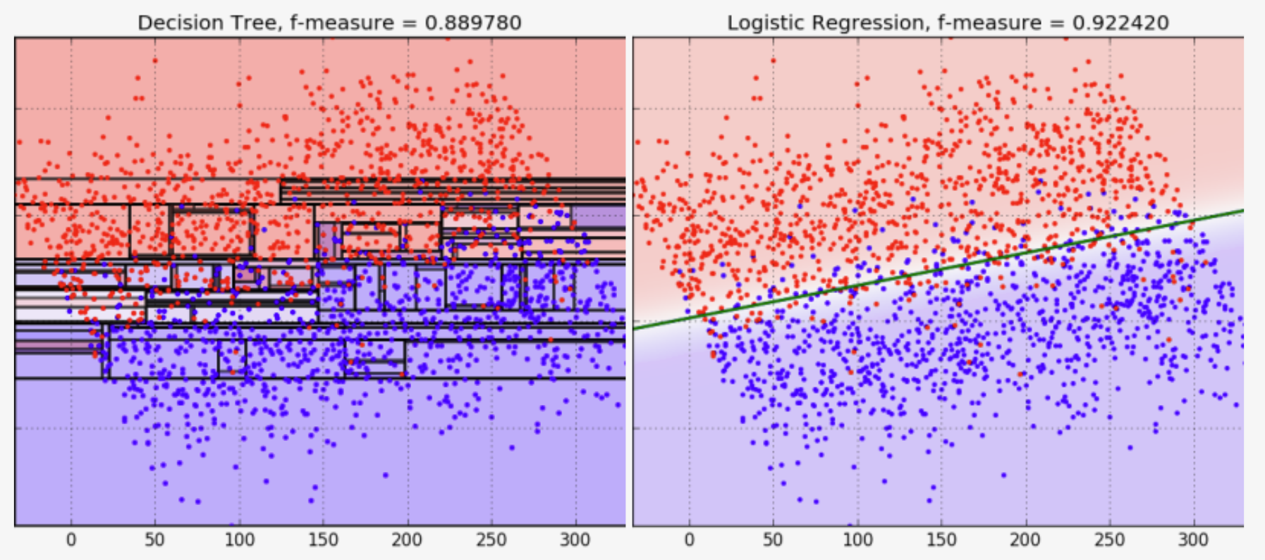
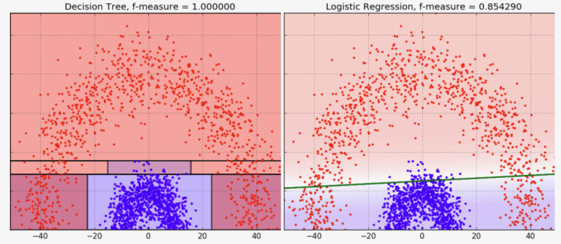
In the picture above, the decision tree is overfit, and has too many specifics and conditions (branches and nodes) that looses a lot in accuracy. The logistic regression handled better this situation. In the picture below, the opposite happened.
Splitting criterias
The criterias are what help the algorith choosing to go one branch or another. There are many but the 3 main ones are:
Gini Impurity measures how often the value would be wrongly classified if the decision was made randomly. How impure is a nod.
\[I_G(n)=1-\sum_{i=1}^{J}(p_i)^2\]Entropy measures the tidyness of a system in a dataset and helps choosing the value that brings most gain of information (the decision made in the root node)
\[Entropy=\sum_{i=1}^C-p_i*log_2(p_i)\]Variance is used in regression models. Should remain low to avoid overfitting the model.
\[Variance=\frac{\sum(X-\overline{X})^2}{n}\]Implementation
With Python and SciKitLearn it is easy to create a machine learning model using a decision tree. There are many datasets available online to test it out.
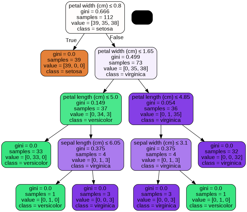
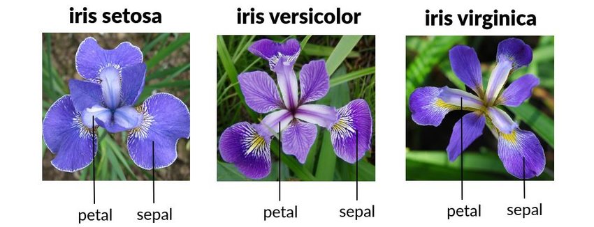
Start by importing pandas and numpy. The datasaet can be imported from scikit directly. The iris dataset is made of 150 lines for 4 columns that contain the size (length and width) of sepals and petals, that help determine the class of the iris, as follows:
Import packages and load data
import pandas as pd
import numpy as np
from sklearn.datasets import load_iris
data = load_iris()
The data is now loaded in Colab. We need to identify where is the data used to guess, and where are the labels (answers) for the training part:
X = data.data
y = data.target

from sklearn.model_selection import train_test_split
X_train,X_test,y_train,y_test = train_test_split(X,y,random_state=50,test_size=0.25)

from sklearn import tree
clf = tree.DecisionTreeClassifier(random_state=50)
This where we give parameters to build the model. Because of the nature of decison trees a certain randomness in the branch making is required. Any number works, but different ones at each training will give verying results. The test sample size is 25% of the total dataset. 75% of the dataset will be used for training.
Have a look at the tree parameters
The get_params() method allows to have a glimpse at the parameters set for this tree. Here we have :
parameters = pd.Series(clf.get_params()).to_frame('Value')
print('Tree parameters:\n',parameters)
| Tree parameters | Value |
|---|---|
| ccp_alpha | 0 |
| class_weight | None |
| criterion | gini |
| max_depth | None |
| max_features | None |
| max_leaf_nodes | None |
| min_impurity_decrease | 0 |
| min_samples_leaf | 1 |
| min_samples_split | 2 |
| min_weight_fraction_leaf | 0 |
| random_state | 50 |
| splitter | best |
The splitting criterion is Gini by default.
Test the model and see its accuracy
clf.fit(X_train,y_train)
y_pred = clf.predict(X_test)

from sklearn.metrics import accuracy_score

print('Accuracy of the training data (Gini):', accuracy_score(y_true=y_train, y_pred=clf.predict(X_train)))
print('Accuracy of the testing data (Gini):',accuracy_score(y_true=y_test,y_pred=y_pred))
print('\n')
Results:
Accuracy of the training data (Gini): 1.0
Accuracy of the testing data (Gini): 0.9473684210526315
So next time we feed data bout length and width of Iris, This model can tell with 94.74% accuracy wether it is Setosa, Versicolor or Virginica.
To test the model with an Entropy splitting criterion, or others, you can edit this line of code tree.DecisionTreeClassifier(random_state=50) to tree.DecisionTreeClassifier(random_state=50,criterion = 'entropy'.
Visualization
We can also visualize the tree with a little more code:
!pip install pydotplus
from sklearn.tree import export_graphviz
from six import StringIO
from IPython.display import Image
import pydotplus

dot_data = StringIO()
export_graphviz(clf, out_file=dot_data,
                filled=True, rounded=True,
                special_characters=True,feature_names = data.feature_names,class_names=data.target_names)
graph = pydotplus.graph_from_dot_data(dot_data.getvalue())
Image(graph.create_png())
Result: