오늘은 RNN 모델중 하나인 LSTM을 통해 삼성전자 주가를 예측해보겠습니다.

데이터셋 생성

데이터셋을 다운로드 하고자 하는 경우 링크에 접속하여 받을 수 있습니다.

df_price = pd.read_csv(os.path.join(data_path, '01-삼성전자-주가.csv'), encoding='utf8')
df_price.describe()

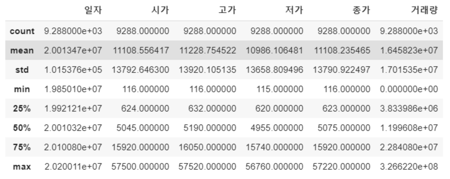
컬럼은 일자, 시가, 고가, 저가, 종가, 거래량으로 구성 되어있으며 총 9,288개의 record를 갖고 있습니다.
해당 데이터 스키마를 갖고 미래 특정 시점의 ‘종가’를 예측해보겠습니다.

import numpy as np # linear algebra  
import pandas as pd # data processing, CSV file I/O (e.g. pd.read_csv)  
import matplotlib.pyplot as plt  
import seaborn as sns  

데이터 전처리 및 시각화

날짜형 변환(-> datetime)

pd.to_datetime(df_price['일자'], format='%Y%m%d')
# 0      2020-01-07
# 1      2020-01-06
# 2      2020-01-03
# 3      2020-01-02
# 4      2019-12-30

df_price['일자'] = pd.to_datetime(df_price['일자'], format='%Y%m%d')
df_price['연도'] =df_price['일자'].dt.year
df_price['월'] =df_price['일자'].dt.month
df_price['일'] =df_price['일자'].dt.day

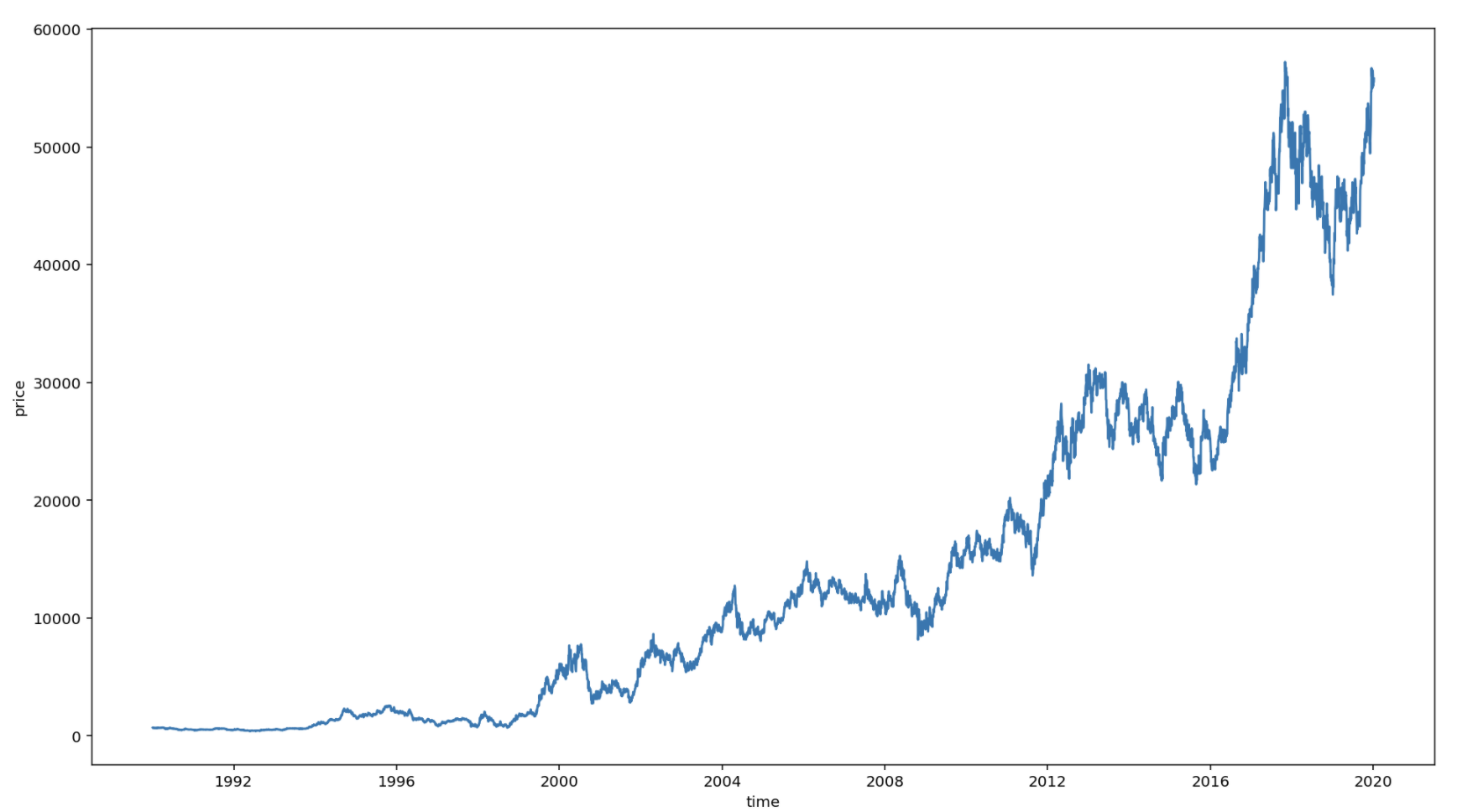
1990년도 이후 주가 시각화

df = df_price.loc[df_price['연도']>=1990]

plt.figure(figsize=(16, 9))
sns.lineplot(y=df['종가'], x=df['일자'])
plt.xlabel('time')
plt.ylabel('price')

데이터 정규화

딥러닝 모델 학습을 원활히 하기 위해 독립변수와 종속변수를 정규화해준다.

from sklearn.preprocessing import MinMaxScaler

scaler = MinMaxScaler()
scale_cols = ['시가', '고가', '저가', '종가', '거래량']
df_scaled = scaler.fit_transform(df[scale_cols])

df_scaled = pd.DataFrame(df_scaled)
df_scaled.columns = scale_cols

print(df_scaled)

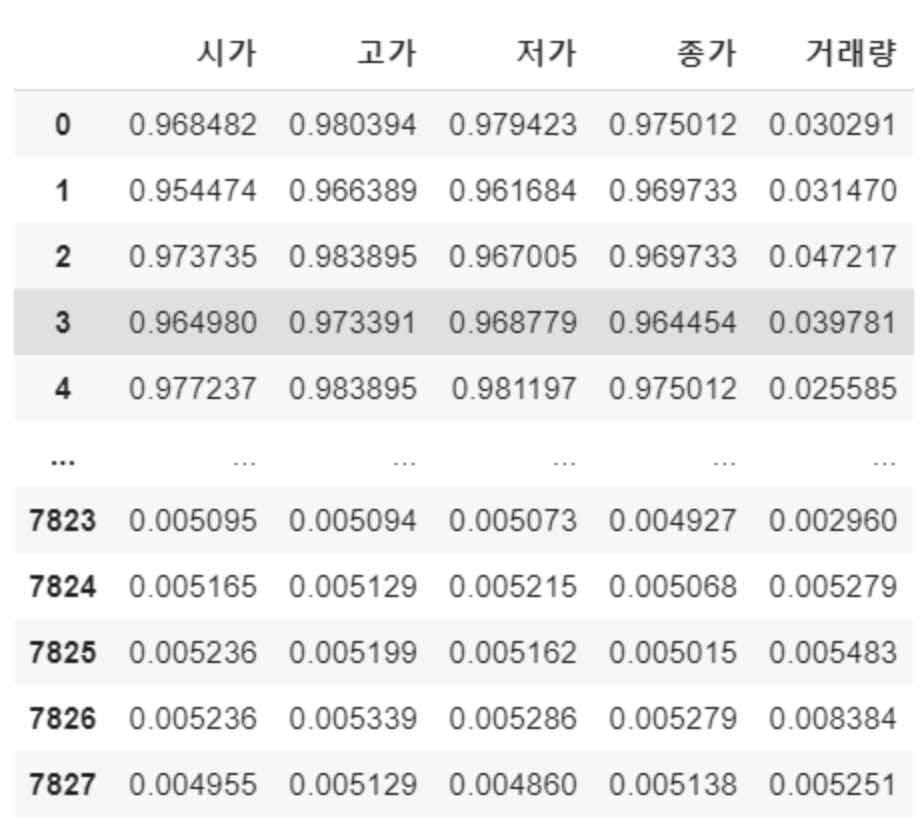
모든 컬럼의 스케일이 0~1로 변경되어 출력된 모습

학습 데이터셋 생성

window_size를 정의하여 학습 데이터를 생성합니다.
window_size는 내가 얼마동안(기간)의 주가 데이터를 기반으로 다음날 종가를 예측할 것인가를 정하는 파라미터입니다.
GCP AutoML에서의 historical data feed size와 동일한 개념입니다.
해당 예제에서는 과거 20일을 기준으로 그 다음날의 데이터를 예측해보겠습니다.

TEST_SIZE = 200
WINDOW_SIZE = 20

train = df_scaled[:-TEST_SIZE]
test = df_scaled[-TEST_SIZE:]

dataset 만들어주는 함수 작성

def make_dataset(data, label, window_size=20):
    feature_list = []
    label_list = []
    for i in range(len(data) - window_size):
        feature_list.append(np.array(data.iloc[i:i+window_size]))
        label_list.append(np.array(label.iloc[i+window_size]))
    return np.array(feature_list), np.array(label_list)

위 함수는 정해진 window_size에 기반해서 20일 기간의 데이터셋을 묶어주는 함수입니다.
순차적으로 20일 동안의 데이터셋을 묶고, 이에 맞는 label을 매핑하여 return 해줍니다.

feature와 label 정의

feature_cols = ['시가', '고가', '저가', '거래량']
label_cols = ['종가']

train_feature = train[feature_cols]
train_label = train[label_cols]

# train dataset
train_feature, train_label = make_dataset(train_feature, train_label, 20)

# train, validation set 생성
from sklearn.model_selection import train_test_split
x_train, x_valid, y_train, y_valid = train_test_split(train_feature, train_label, test_size=0.2)

x_train.shape, x_valid.shape
# ((6086, 20, 4), (1522, 20, 4))

# test dataset (실제 예측 해볼 데이터)
test_feature, test_label = make_dataset(test_feature, test_label, 20)
test_feature.shape, test_label.shape
# ((180, 20, 4), (180, 1))

LSTM 모델 생성

from keras.models import Sequential
from keras.layers import Dense
from keras.callbacks import EarlyStopping, ModelCheckpoint
from keras.layers import LSTM

model = Sequential()
model.add(LSTM(16, 
               input_shape=(train_feature.shape[1], train_feature.shape[2]), 
               activation='relu', 
               return_sequences=False)
          )
model.add(Dense(1))

모델 학습

model.compile(loss='mean_squared_error', optimizer='adam')
early_stop = EarlyStopping(monitor='val_loss', patience=5)
filename = os.path.join(model_path, 'tmp_checkpoint.h5')
checkpoint = ModelCheckpoint(filename, monitor='val_loss', verbose=1, save_best_only=True, mode='auto')

history = model.fit(x_train, y_train, 
                    epochs=200, 
                    batch_size=16,
                    validation_data=(x_valid, y_valid), 
                    callbacks=[early_stop, checkpoint])

# ...
# ...

# Epoch 00015: val_loss did not improve from 0.00002
# Epoch 16/200
# 6086/6086 [==============================] - 12s 2ms/step - loss: 3.1661e-05 - val_loss: 4.1063e-05

# Epoch 00016: val_loss did not improve from 0.00002
# Epoch 17/200
# 6086/6086 [==============================] - 13s 2ms/step - loss: 2.4644e-05 - val_loss: 4.0085e-05

# Epoch 00017: val_loss did not improve from 0.00002
# Epoch 18/200
# 6086/6086 [==============================] - 13s 2ms/step - loss: 2.2936e-05 - val_loss: 2.4692e-05

# Epoch 00018: val_loss did not improve from 0.00002

Early Stop 옵션으로 인해 18번째 Epoch 기준 0.00002의 평균오차에서 학습이 포화되어 중단됐습니다.
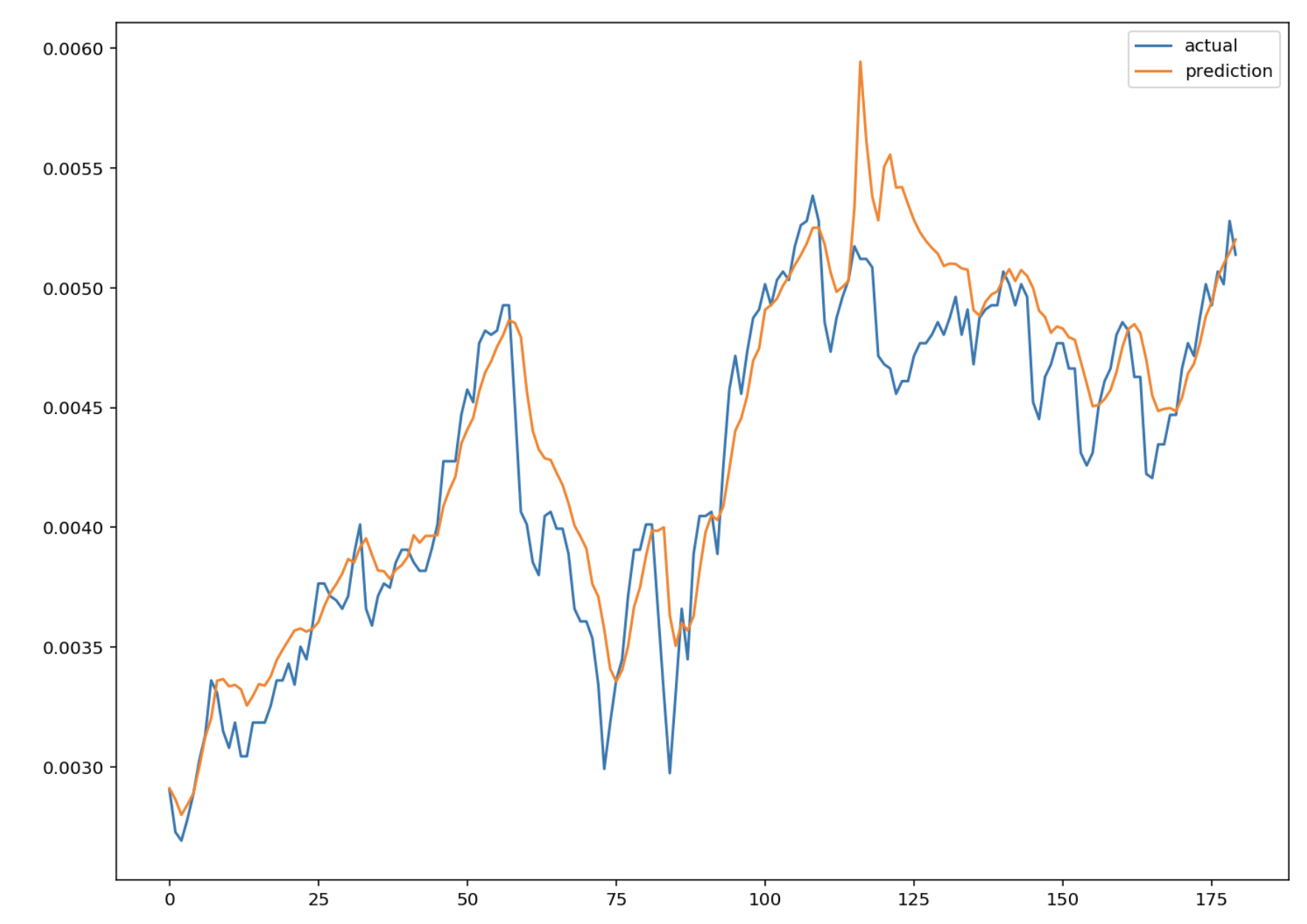
다음으로 학습한 모델로 미래 주가 예측을 해보겠습니다.

# weight 로딩
model.load_weights(filename)

# 예측
pred = model.predict(test_feature)

실제 데이터와 예측한 데이터 시각화

((6086, 20, 4), (1522, 20, 4))

plt.figure(figsize=(12, 9))
plt.plot(test_label, label='actual')
plt.plot(pred, label='prediction')
plt.legend()
plt.show()

Reference

Lee, T. (2020, February 14). 딥러닝(LSTM)을 활용하여 삼성전자 주가 예측을 해보았습니다.
Retrieved August 27, 2020, from https://teddylee777.github.io/tensorflow/LSTM으로-예측해보는-삼성전자-주가